4. Python Tutorials

These tutorials are written in Jupyter, but you can also run them in ipython if you prefer. For Jupyter, we need to set the options below, but if you are running only ipython, instead of %matplotlib inline try using %matplotlib qt5 or %matplotlib osx, depending on your system.

You should start Python in the directory where you have the IRIS-9 data (e.g. ~/iris9/ as we defined earlier).

%matplotlib inline
import numpy as np
import astropy.io.fits as fits
import matplotlib.pyplot as plt
from astropy.wcs import WCS
# Set up some default matplotlib options
plt.rcParams['figure.figsize'] = [10, 6]
plt.rcParams['xtick.direction'] = 'out'
plt.rcParams['image.origin'] = 'lower'
plt.rcParams['image.cmap'] = 'viridis'

4.1. Mg II Dopplergrams

In this tutorial we are going to produce a Dopplergram for the Mg II k line from an IRIS 400-step raster. The Dopplergram is obtained by subtracting the intensities at symmetrical velocity shifts from the line core (e.g. ±50 km/s). For this kind of analysis we need a consistent wavelength calibration for each step of the raster.

This very large dense raster took more than three hours to complete the 400 scans (30 s exposures), which means that the spacecraft’s orbital velocity changes during the observations. This means that any precise wavelength calibration will need to correct for those shifts.

Let’s open the file:

iris_file = fits.open("iris_l2_20140708_114109_3824262996_raster_t000_r00000.fits",
                 memmap=True, do_not_scale_image_data=True)

Here we use memmap to save memory.

We can now print out the spectral windows in the file:

hd = iris_file[0].header
print('Window. Name      : wave start - wave end\n')
for i in range(hd['NWIN']):
    win = str(i + 1)
    print('{0}. {1:15}: {2:.2f} - {3:.2f} Å'
          ''.format(win, hd['TDESC' + win], hd['TWMIN' + win], hd['TWMAX' + win]))

Window. Name      : wave start - wave end

1. C II 1336      : 1332.70 - 1337.58 Å
2. Fe XII 1349    : 1347.68 - 1350.90 Å
3. O I 1356       : 1352.25 - 1356.69 Å
4. Si IV 1394     : 1390.90 - 1396.19 Å
5. Si IV 1403     : 1398.63 - 1406.34 Å
6. 2832           : 2831.23 - 2834.26 Å
7. 2814           : 2812.54 - 2816.41 Å
8. Mg II k 2796   : 2792.98 - 2806.63 Å

We see that Mg II is in window 8, so let’s load those data and get the WCS information to construct the wavelength arrays and get coordinates:

data = iris_file[8].data
wcs = WCS(iris_file[8].header)

And let’s calculate the wavelength array:

m_to_nm = 1e9  # convert wavelength to nm
wave = wcs.all_pix2world(np.arange(wcs._naxis[0]), [0.], [0.], 1)[0] * m_to_nm

We can see how the the spatially averaged spectrum looks like:

plt.plot(wave, data.mean((0, 1)))

[<matplotlib.lines.Line2D at 0xa80fe2128>]

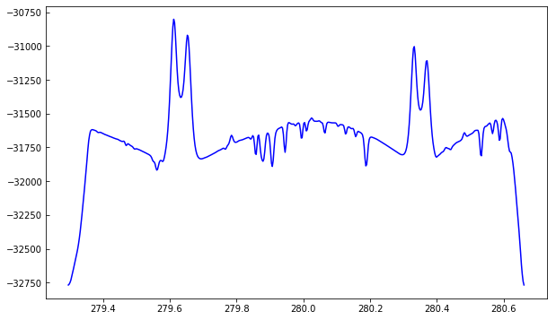
Because we used memmap, the intensity values are unscaled and do not represent the IRIS data number (DN). For the purposes of this tutorial this is not a problem.

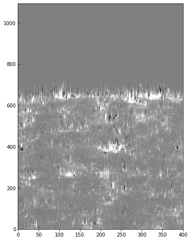
To better understand the orbital velocity problem let us look at how the line intensity varies for a strong Mn I line at around 280.2 nm, in between the Mg II k and h lines. For this dataset, the line core of this line falls around index 350. To plot a spectroheliogram in the correct orientation we will transpose the data:

fig = plt.figure(figsize=(6, 10))
plt.imshow(data[..., 350].T, vmin=-32000, vmax=-31600, aspect=0.5)

<matplotlib.image.AxesImage at 0xa8114ffd0>

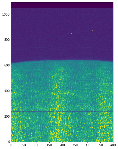
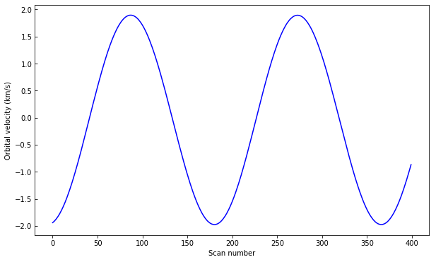
You can see a regular bright-dark pattern along the x axis, an indication that its intensities are not taken at the same position in the line because of wavelength shifts. The shifts are caused by the orbital velocity changes, and we can find these in the auxiliary metadata:

aux = iris_file[-2]
v_obs = aux.data[:, aux.header['OBS_VRIX']]
v_obs /= 1000.  # convert to km/s
plt.plot(v_obs)
plt.ylabel("Orbital velocity (km/s)")
plt.xlabel("Scan number")

Text(0.5,0,'Scan number')

To look at intensities at any given scan we only need to subtract this velocity shift from the wavelength scale, but to look at the whole image at a given wavelength we must interpolate the original data to take this shift into account. Here is a way to do it (note that array dimensions apply to this specific set only!):

from scipy.constants import c
from scipy.interpolate import interp1d
c_kms = c / 1000.
wave_shift = - v_obs * wave[350] / (c_kms)
# linear interpolation in wavelength, for each scan
for i in range(iris_file[0].header['NRASTERP']):
    tmp = interp1d(wave - wave_shift[i], data[i], bounds_error=False)
    data[i] = tmp(wave)

And now we can plot the shifted data to see that the large scale shifts have disappeared:

fig = plt.figure(figsize=(6, 10))
plt.imshow(data[..., 350].T, vmin=-32000, vmax=-31600, aspect=0.5)

<matplotlib.image.AxesImage at 0xa82540278>

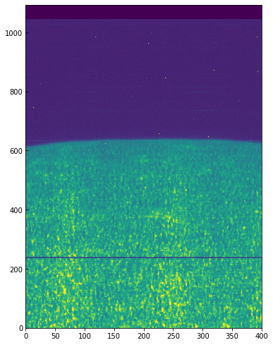
Some residual shift remains, but we will not correct for it here. A more elaborate correction can be obtained by the IDL routine iris_prep_wavecorr_l2, but this has not yet been ported to Python see the IDL version of this tutorial for more details.

We can use the calibrated data for example to calculate Dopplergrams. A Dopplergram is here defined as the difference between the intensities at two wavelength positions at the same (and opposite) distance from the line core. For example, at +/- 50 km/s from the Mg II k3 core. To do this, let us first calculate a velocity scale for the k line and find the indices of the -50 and +50 km/s velocity positions (here using the convention of negative velocities for up flows):

mg_k_centre = 279.63521  # in nm
pos = 50  # in km/s around line centre
velocity =  (wave - mg_k_centre) * c_kms / mg_k_centre
index_p = np.argmin(np.abs(velocity - pos))
index_m = np.argmin(np.abs(velocity + pos))
doppl = data[..., index_m] - data[..., index_p]

And now we can plot this as before (intensity units are again arbitrary because of the unscaled DNs):

fig = plt.figure(figsize=(6, 10))
plt.imshow(doppl.T, cmap='gist_gray', aspect=0.5,
           vmin=-700, vmax=700,)

<matplotlib.image.AxesImage at 0xa82bf4908>

4.2. Flare 4-step raster: SJI and spectrograph

This exercise will be solved mostly by the participants. The low-level guide to IRIS with Python will serve as a reference for most of the tasks necessary to complete this exercise.

In this exercise we will combine the slit-jaw and spectrograph images taken during a small flare. The data are from 2014-11-07, with file names iris_l2_20141107_160734_3860258971_*. The programme was a 4-step raster, and there are 80 repeats. In the files provided there is only the 2796 slit-jaw.

Start by loading the slit-jaw file and then do the following:

• Find out what is the timestep at 2014-11-07T16:19:07.800. Remember that just like in the raster files, the array with times is saved in the second to last extension of the SJI fits files. Plot the SJI image at that timestep, in solar (x, y) coordinates in arcsec.
• Did the exposure time vary for this slit-jaw file? Ie, was the Auto Exposure Compensation (AEC) triggered? Check the second to last extension in the file, the data column number for exposure times is saved in the keyword EXPTIMES in the second to last extension.
• Check what is the closest raster file for the time of 2014-11-07T16:19:07.800. Load that file, and check the spectra for the window Si IV 1403. Was the exposure saturated at any position?
• Get the solar y coordinates (in arcsec) of the slit using the WCS information in the header of the loaded raster file. Hint 1: this can be obtained in a similar way as we obtain the wavelength from the WCS header, but for the y coordinate we need to get the second WCS coordinate, e.g.: y = wcs.all_pix2world([0.], np.arange(N_PIX_SLIT), [0.], 0)[1]. Hint 2: note that astropy’s WCS internally uses degrees as unit for the radial coordinates. If you just print the wcs object, you will see that in this case that CRVAL[2] = -0.1672825 (in degrees), which is about -10’ (you can also check this in the SJI plot).
• You can now put everything together and make an image plot (imshow) of the Si IV 1403, using the solar y scale on the y axis and the wavelength scale on the x axis, for any of the raster positions. To do this you supply the keyword argument extent to imshow, e.g.: extent=[wavelength.min(), wavelength.max(), y.min(), y.max()]. The results should be something like:

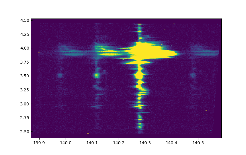
Si IV 1403