3. IDL Tutorials¶

3.1. IRIS xfiles¶

This tutorial will guide you step-by-step into some features of iris_xfiles, a quicklook tool. Go to the directory with the IRIS data, start IDL as described above, and then start iris_xfiles:

IDL> iris_xfiles

Note

It is important that you start IDL on the ~/iris9/ directory, and from the command line. Not doing so will result in files you create later being saved in a different directory, and some of the instructions here will not be correct. If you do not run IDL from the ~/iris9/ directory, make note of where you run it from, so you can find your files later on.

In the middle panel, next to Search Directory: press Change. Then navigate to the directory ~/iris9, press OK when this directory is selected. Notice that Search Pattern changed to free search. Then change Start Time to 01-Aug-2012 00:00:00 and press Up until now to change the Stop Time to the current time. This will ensure that the search covers all the observation dates from the files we have.

Now press Start Search, and you should see the list of observations appear. To save disk sapce, the data in the tutorial materials is incomplete (ie, some observations only have the spectrograph files, others have only some of the SJI files). Navigate through the observations (and their files in the pane below) to find some with SJI files. Use iris_xfiles to look at some SJI movies.

Now load the dataset from 2013-12-26 and open the raster file. What can you say about the line list? Make a movie of the Mg II k spectra and explore them. Finally, generate level 3 files, selecting the Si IV 1403 and Mg II k 2796 lines. In the next dialog, uncheck all the options. We will use these later with CRISPEX. Note that no sp file was created, as these observations comprise only a single 400-step raster.

Note

The profile moments in Line fit is not currently working. You can also explore the data using single or double Gauss fit options, but for this raster doing the Gaussian fits may take between 30-60 minutes, depending on your laptop.

3.2. Mg II Dopplergrams¶

In this tutorial we are going to produce a Dopplergram for the Mg II k line from an IRIS 400-step raster. The Dopplergram is obtained by subtracting the intensities at symmetrical velocity shifts from the line core (e.g. ±50 km/s). For this kind of analysis we need a consistent wavelength calibration for each step of the raster.

We will use the dataset from 2014-11-07. Feel free to examine these data in iris_xfiles. This very large dense raster took more than three hours to complete the 400 scans (30 s exposures), which means that the orbital velocity and thermal drifts were changed during the observations. Any precise wavelength calibration will need to correct for those shifts. In most cases, level 2 data have already been corrected for these shifts, but this example shows a dataset for which the automatic calibration still left a residual shift that we must correct for.

First lets load the data using the IDL object interface:

IDL> filename = 'iris_l2_20140708_114109_3824262996_raster_t000_r00000.fits'
IDL> d = iris_obj(filename)

Let us see the lines that are saved in this raster:

IDL> d->show_lines
Spectral regions(windows)
 1335.71   C II 1336
 1349.43   Fe XII 1349
 1355.60   O I 1356
 1393.78   Si IV 1394
 1402.77   Si IV 1403
 2832.70   2832
 2814.43   2814
 2796.20   Mg II k 2796

Let us load the Mg II k line into memory:

IDL> wave = d->getlam(7)
IDL> data = d->getvar(7, /load)

We can see how the the spatially averaged spectrum looks like:

IDL> mspec = total(total(data, 2), 2)
IDL> plot, wave, mspec
IDL> plot, wave, mspec, xrange=[2794, 2799], /xst

To better understand the orbital velocity problem let us look at how the line intensity varies for a strong Mn I line at around 280.2 nm, in between the Mg II k and h lines. For this dataset, the line core of this line falls around index 350. To plot it in the correct orientation we will make use of IDL’s rotate, and the procedure pih (available in the IRIS tree of solarsoft) to make the plot:

IDL> pih, rotate(reform(data[350, *, *]), 1), min=0, max=120, scale=[0.35, 0.1667]

The result should look like this:

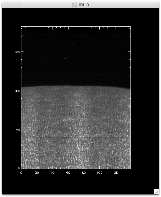
Intensity at Mn I 280.2 nm line when orbital velocity and thermal drifts are not fully accounted for.

You can see that the left side of the figure is brighter, and indication that its intensities are not taken at the same position in the line because of wavelength shifts.

To calculate the wavelength shifts from the orbital velocity and thermal drifts we do the following:

IDL> wavecorr = iris_prep_wavecorr_l2(filename)

This routine measures the wavelength position of 5 neutral lines (3 NUV, 2 FUV) whose rest wavelengths are reasonably well known, and saves the shifts (in Ångström) into the structure variable called wavecorr.

The wavelength shift in the i-th line in the j-th frame of the k-th input file is stored in wavecorr.corrs[k, j, i] . Averaged and smoothed corrections for the NUV and FUV are stored in corr_nuv and corr_fuv. To plot the per-frame measured wavelength shift and the smoothed correction in the NUV and FUV one would do:

IDL> utplot, wavecorr.times, wavecorr.corrs[0,*,0], psym = 4, chars = 1.5, title = 'NUV', ytitle = 'Wavelength shift [A]', /xst
IDL> outplot, wavecorr.times, wavecorr.corr_nuv, col = 200, thick = 2

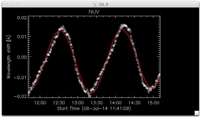
Fit to the orbital velocity/thermal shifts from iris_prep_wavecorr_l2. Your colours may appear different from this figure, depending on which color table you loaded.

To look at intensities at any given scan we only need to subtract this shift from the wavelength scale, but to look at the whole image at a given wavelength we must interpolate the original data to take this shift into account. Here is a way to do it (note that array dimensions apply to this specific set only!):

IDL> new_data = fltarr(537, 1095, 400, /n)
IDL> ; subtract mean shift
IDL> wavecorr.corr_nuv = wavecorr.corr_nuv - mean(wavecorr.corr_nuv)
IDL> .r
for i=0, 399 do begin
   for j=0, 1094 do begin
       new_data[*, j, i] = interpol(data[*, j, i], wave + wavecorr.corr_nuv[i], wave)
   endfor
endfor
end

(This double loop will take a while to complete.)

Once you have the calibrated data, we can compare again how it looks at the Mn I line wavelength:

IDL> pih, rotate(reform(new_data[350, *, *]), 1), min=0, max=120, scale=[0.35, 0.1667]

And now we can see that the intensity map is uniform along the solar disk:

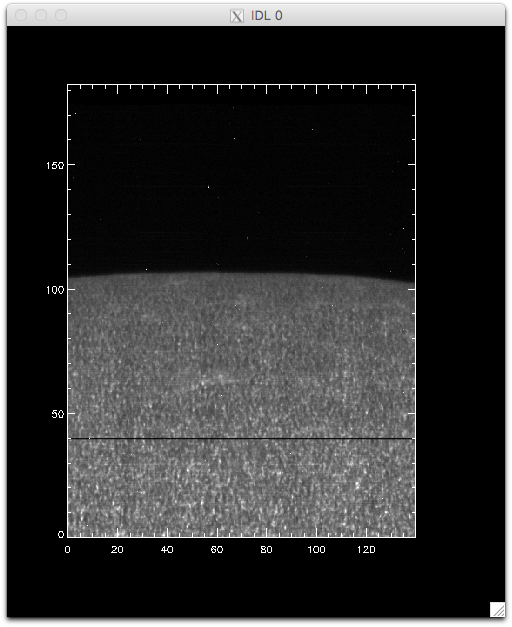
Intensity at Mn I 280.2 nm line when orbital velocity and thermal drifts are accounted for.

We can use this calibrated data for example to calculate dopplergrams. A dopplergram is the difference between the intensities at two wavelength positions at the same (and opposite) distance from the line core. For example, at +/- 50 km/s from the Mg II k3 core. To do this, let us first calculate a velocity scale for the k line and find the indices of the -50 and +50 km/s velocity positions:

IDL> k_centre = 2796.3521
IDL> vel = (k_centre - wave) * 3e5 / k_centre
IDL> ; find approximate index of -50 and 50 km/s
IDL> tmp = min(abs(vel - 50), i50p)
IDL> tmp = min(abs(vel + 50), i50m)

Now get the dopplergram and plot it:

IDL> doppgr = rotate(reform(new_data[i50m, *, *] - new_data[i50p, *, *]), 1)
IDL> pih, doppgr, min=-100, max=100, scale=[0.35, 0.1667]

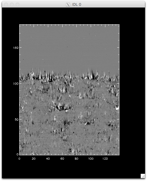
Dopplegram for Mg II k at +/- 50 km/s.

3.3. CRISPEX¶

Warning

The version of CRISPEX in the reduced version of SolarSoft we provide has a bug and fails with 400-step rasters. Please download the latest version of CRISPEX , and unpack the tar file into the correct directory by doing: tar zxvf crispex_v1.7.4.13.tar.gz -C ~/iris9/ssw/iris/idl/uio/.

3.3.1. Active region 400-step raster¶

Let us go back to the first dataset we worked with, and run CRISPEX on the level 3 file:

IDL> crispex, 'iris_l3_20131226_171752_3840007146_t000_SiIV1403_MgIIk2796_im.fits'

Note

If you haven’t created the level 3 file with iris_xfiles, you can create it quickly from the IDL command line (assuming you are at the directory with the level 2 files):

IDL> f = iris_files('iris_l2_20131226*raster*')
IDL> iris_make_fits_level3, f, [1, 3]

Explore the dataset with CRISPEX, and go through the following tasks/questions:

Adjust the scaling of the spectral plot so that the lines are visible (Displays tab, lower/upper y-values, and also multipliers in Scaling tab under Detailed spectrum)
Look at the main image in the cores of the Mg II k and Si IV lines. Adjust scaling for Si IV 1403 so that it becomes visible (change Histogram optimisation to 0.001 and/or set gamma lower than 1)
Blink the image between the spectral positions of the cores of the Si IV and Mg II k lines (use animation speed of about 2 frames/s)
Can you find a large dot where Si IV is greatly enhanced but Mg II is not too unusual? What are its solar (x, y) coordinates?
Is there a sunspot or a pore in these observations? How do you find out?

3.3.2. Flare 4-step raster¶

Now let us look at a different type of IRIS observation, a 4-step dense raster with 80 repeats during which a flare was caught. First, we need to produce the level 3 files for this dataset, so let us do that from IDL:

IDL> f = iris_files('iris_l2_20141107*raster*')
IDL> ; make level 3 files with C II, Si IV, and Mg II (indices 0, 4, 8)
IDL> iris_make_fits_level3, f, [0, 4, 8], /sp

Let us now run CRISPEX using both im and sp files, and also use a slit-jaw image:

IDL> l3files = iris_files('iris_l3_20141107*')
IDL> sji = iris_files('iris_l2_20141107*SJI*')
IDL> crispex, l3files[0], l3files[1], sjicube=sji[0]

When CRISPEX opens, you can see multiple windows, including the slit-jaw image with the 4 raster positions superimposed.

In CRISPEX the visualisation of this dataset has both a time domain and a main image with 16 columns. Feel free to explore this dataset, first by creating the level 3 files and loading them in CRISPEX. When used with a sjicube option, one can see the 4 positions superimposed in the slit-jaw image.

Explore the dataset with CRISPEX, and go through the following tasks/questions:

Start running the time sequence. At what time does this observation finish?
Is there a sympathetic flare in the same region?
Adjust the slit-jaw image scaling so you can see more than the flare ribbons
At frame 48, the slit-jaw image overall intensity gets much lower. Why is that?
Show only the Mg II lines (Diagnostics tab, unselect other lines and then Spectral tab, narrow down Doppler minimum/maximum values)
Lock the mouse at a given position, see how the temporal evolution goes through the Spectral T-slice window
Can you find a location with the Mg II triplet lines in emission?