3. Tutorials¶

3.1. Preparation¶

The data files for these tutorials were hopefully passed on to participants before. Otherwise, they can be downloaded from http://folk.uio.no/tiago/iris7/IRISdata.zip. This file contains several datasets from IRIS. Throughout the tutorials it is assumed that this file is unpacked into a directory in your home directory named data_temp/. If you want to use a different directory, just replace the name when necessary.

To start, create a directory called data_temp and unzip the data in there. In the Unix terminal, you can do it like this:

% mkdir ~/data_temp
% cp IRISdata.zip ~/data_temp
% cd ~/data_temp
% unzip IRISdata.zip
(...)

Make sure you are in the same directory as the IRISdata.zip file. This will create a directory ~/data_temp/iris with three subdirectories, one per dataset.

You will need to make sure that you have an up-to-date version of SolarSoft IDL with the IRIS branch. You’ll need to have included iris in the SSW_INSTR environment variable, e.g.:

setenv SSW_INSTR "sot iris ontology"

If you have a working version of SolarSoft with the IRIS package you don’t need to do anything else.

It is outside the scope of these tutorials to help you install and configure SolarSoft. If you don’t have it already in your system we provide a tar file with a minimal version that can be used to run the tutorials. This minimal version of SolarSoft has not been tested in many platforms, and is not guaranteed to work. It should be used as a last resort only for those who didn’t have time to do a proper installation. To install it, download the file http://folk.uio.no/tiago/iris5/ssw_iris_minimal.tar.bz2 (483 Mb) and unpack it to your home directory:

tar jxvf ssw_iris_minimal.tar.bz2 -C ~/

(Again we assume the you are in the same directory as the file) This will create a directory ~/ssw with an installation of SolarSoft. Now configure the startup file for your shell, typically ~/.cshrc or ~/.tcshrc (you MUST use csh or tcsh – bash et al. will not work). Add the following lines to your configuration file:

setenv SSW $HOME/ssw
setenv SSW_INSTR "sot iris ontology"

After that, start a new shell and type sswidl. If all went well you have SolarSoft working and are ready to run the tutorials!

3.2. IRIS xfiles¶

This tutorial will guide you step-by-step into some features of iris_xfiles, a quicklook tool. Go to the directory with the IRIS data, open solarsoft IDL and launch iris_xfiles:

% cd ~/data_temp/iris
% sswidl
(...)
IDL> iris_xfiles

In the middle panel, next to Search Directory: press Change. Then navigate to the directory ~/data_temp/iris/20131226_171752_3840007146, press OK when this directory is selected. Notice that Search Pattern changed to free search. Make sure the time of these observations (2013 December 26, 17:17 UT) is contained in between the Start Time and Stop Time range, adjust if necessary.

Now press Start Search, and you should see the list of files appear. Feel free to check the slit-jaw movies and then double click on the raster file. What can you say about the line list?

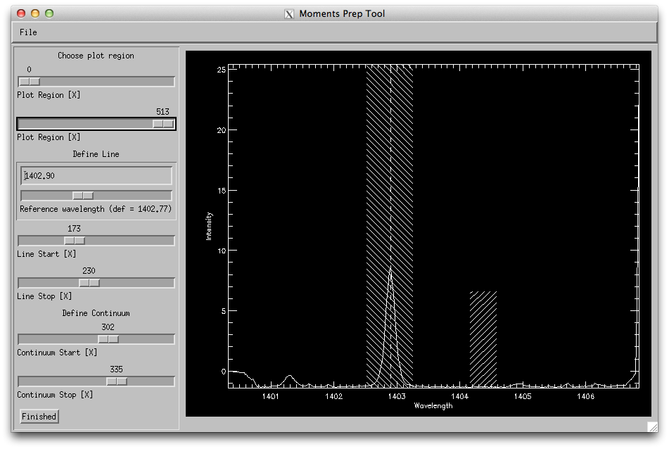
How the wavelength selection iris_xfiles moment tool should look like.

Select the Si IV 1403 line and under Line fit select Profile Moments. On the Moments Prep Tool window adjust the reference wavelength so that it matches the core of the line, and set the line start and stop so that it covers the line. Set the continuum to be about 5-10 pixels wide on a region with no lines. Press Finished (and wait a while...). What do you see?

The result for intensity should look like this (set log(HistoOpt Value) to -1.65):

Now select the Mg II k 2796 line instead, and choose again Profile moments. Set the line start and stop so that it is about 5 pixels wide around k3. Set the continuum to be about 5 pixels wide on the right side of the plot, in a region with no absorption lines. The result for intensity should look like this:

Go back to the IRIS_Xcontrol window of the raster file. Select the Si IV 1403 and Mg II k 2796 lines and press Generate level3 files. In the next dialog select only add “20131226_171752_3840007146/” to save directory, so that the level 3 file is saved in the existing directory. We will use this level 3 file later with CRISPEX. Note that no sp file was created, as these observations comprise only a single 400-step raster.

3.3. Mg II Dopplergrams¶

In this tutorial we are going to produce a Dopplergram for the Mg II k line from an IRIS 400-step raster. The Dopplergram is obtained by subtracting the intensities at symmetrical velocity shifts from the line core (e.g. ±50 km/s). For this kind of analysis we need a consistent wavelength calibration for each step of the raster.

The data set directory should be:

IDL> data_dir = '~/data_temp/iris/20140708_114109_3824262996'

Feel free to examine these data in iris_xfiles. This very large dense raster took more than three hours to complete the 400 scans (30 s exposures), which means that the orbital velocity and thermal drifts were changed during the observations. This means that any precise wavelength calibration will need to correct for those shifts. In most cases level 2 data have already been corrected for these shifts, but this example shows a dataset for which the automatic calibration still left a significant component which must be corrected for.

First lets load the data using the IDL object interface:

IDL> filename = 'iris_l2_20140708_114109_3824262996_raster_t000_r00000.fits'
IDL> filename = data_dir + '/' + filename
IDL> d = iris_obj(filename)

Let us see the lines that are saved in this raster:

IDL> d->show_lines
Spectral regions(windows)
0   1335.71   C II 1336
1   1349.43   Fe XII 1349
2   1355.60   O I 1356
3   1393.78   Si IV 1394
4   1402.77   Si IV 1403
5   2832.70   2832
6   2814.43   2814
7   2796.20   Mg II k 2796

Let us load the Mg II k line into memory:

IDL> wave = d->getlam(7)
IDL> data = d->getvar(7, /load)

We can see how the the spatially averaged spectrum looks like:

IDL> mspec = total(total(data, 2), 2)
IDL> plot, wave, mspec
IDL> plot, wave, mspec, xrange=[2794, 2799], /xst

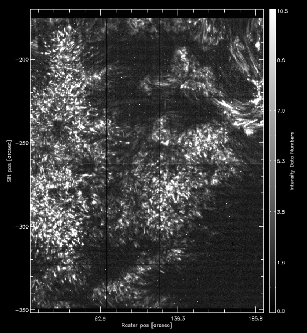
To better understand the orbital velocity problem let us look at how the line intensity varies for a strong Mn I line at around 280.2 nm, in between the Mg II k and h lines. For this dataset, the line core of this line falls around index 350. To plot it in the correct orientation we will make use of IDL’s rotate, and the procedure pih (available in the IRIS tree of solarsoft) to make the plot:

IDL> pih, rotate(reform(data[350, *, *]), 1), min=0, max=200, scale=[0.35, 0.1667]

The result should look like this:

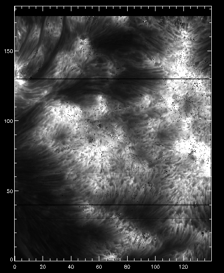
Intensity at Mn I 280.2 nm line when orbital velocity and thermal drifts are not accounted for.

You can see that the left side of the figure is brighter, and indication that its intensities are not taken at the same position in the line because of wavelength shifts.

To calculate the wavelength shifts from the orbital velocity and thermal drifts we do the following:

IDL> wavecorr = iris_prep_wavecorr_l2(filename)

This routine measures the wavelength position of 5 neutral lines (3 NUV, 2 FUV) whose rest wavelengths are reasonably well known, and saves the shifts (in Ångström) into the structure variable called wavecorr.

The wavelength shift in the i-th line in the j-th frame of the k-th input file is stored in wavecorr.corrs[k, j, i] . Averaged and smoothed corrections for the NUV and FUV are stored in corr_nuv and corr_fuv. To plot the per-frame measured wavelength shift and the smoothed correction in the NUV and FUV one would do:

IDL> utplot, wavecorr.times, wavecorr.corrs[0,*,0], psym = 4, chars = 1.5, title = 'NUV', ytitle = 'Wavelength shift [A]', /xst
IDL> outplot, wavecorr.times, wavecorr.corr_nuv, col = 2, thick = 2

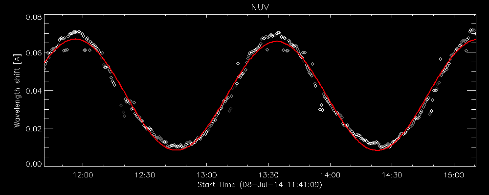
Fit to the orbital velocity/thermal shifts from iris_prep_wavecorr_l2. Your colours may appear different from this figure, depending on which color table you loaded.

To look at intensities at any given scan we only need to subtract this shift from the wavelength scale, but to look at the whole image at a given wavelength we must interpolate the original data to take this shift into account. Here is a way to do it (note that array dimensions apply to this specific set only!):

IDL> new_data = fltarr(536, 1094, 400, /n)
IDL> ; subtract mean shift
IDL> wavecorr.corr_nuv = wavecorr.corr_nuv - mean(wavecorr.corr_nuv)
IDL> .r
for i=0, 399 do begin
   for j=0, 1093 do begin
       new_data[*, j, i] = interpol(data[*, j, i], wave + wavecorr.corr_nuv[i], wave)
   endfor
endfor
end

(This double loop will take a while to complete.)

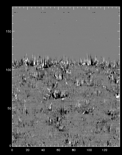
Once you have the calibrated data, we can compare again how it looks at the Mn I line wavelength:

IDL> pih, rotate(reform(new_data[350, *, *]), 1), min=0, max=200, scale=[0.35, 0.1667]

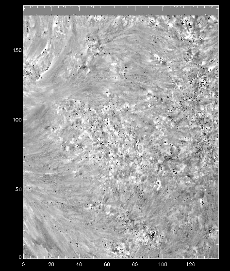
And now we can see that the intensity map is uniform along the solar disk:

Intensity at Mn I 280.2 nm line when orbital velocity and thermal drifts are accounted for.

We can use this calibrated data for example to calculate dopplergrams. A dopplergram is the difference between the intensities at two wavelength positions at the same (and opposite) distance from the line core. For example, at +/- 50 km/s from the Mg II k3 core. To do this, let us first calculate a velocity scale for the k line and find the indices of the -50 and +50 km/s velocity positions:

IDL> k_centre = 2796.31
IDL> vel = (k_centre - wave) * 3e5 / h_centre
IDL> ; find index of -50 and 50 km/s
IDL> tmp = min(abs(vel - 50), i50p)
IDL> tmp = min(abs(vel + 50), i50m)

Now get the dopplergram and plot it:

IDL> doppgr = rotate(reform(new_data[i50m, *, *] - new_data[i50p, *, *]), 1)
IDL> pih, doppgr, min=-80, max=80, scale=[0.35, 0.1667]

Dopplegram for Mg II k at +/- 50 km/s.

3.4. Mg II spectral feature identification¶

In this tutorial we will measure the intensities and velocity shifts of the Mg II k3 and k2 features. We will make use of the iris_get_mg_features_lev2 procedure, which is included in the IRIS SSW package.

Here we will use the same dataset as for the tutorial IRIS xfiles above. The files can be loaded like this:

IDL> data_dir = '~/data_temp/iris/20131226_171752_3840007146'
IDL> filename = 'iris_l2_20131226_171752_3840007146_raster_t000_r00000.fits'
IDL> filename = data_dir + '/' + filename

We can calculate the properties of the Mg II k line in the following manner:

IDL> iris_get_mg_features_lev2, filename, 3, [-40, 40], lc, rp, bp, /onlyk

The output was saved in the arrays lc (line centre), rp (red peak), and bp (blue peak). To save time we calculated only for the k line. We can then visualise both the derived velocities and intensities. For the intensities:

IDL> pih, rotate(reform(lc[0, 1, *, *]), 1), min=0, max=500,  scale=[0.35, 0.1667]
IDL> pih, rotate(reform(bp[0, 1, *, *]), 1), min=0, max=750,  scale=[0.35, 0.1667]
IDL> pih, rotate(reform(rp[0, 1, *, *]), 1), min=0, max=750,  scale=[0.35, 0.1667]

Intensity for the k3 peak from iris_get_mg_features.

and for the velocities:

IDL> pih, rotate(reform(lc[0, 0, *, *]), 1), min=-15, max=15,  scale=[0.35, 0.1667]
IDL> pih, rotate(reform(rp[0, 0, *, *]), 1), min=0, max=30,  scale=[0.35, 0.1667]
IDL> pih, rotate(reform(bp[0, 0, *, *]), 1), min=-30, max=0,  scale=[0.35, 0.1667]

Velocity shifts for the k3 peak from iris_get_mg_features.

3.5. CRISPEX¶

IDL> cd, '~/data_temp/iris/20131226_171752_3840007146'
IDL> crispex, 'iris_l3_20131226_171752_3840007146_t000_SiIV1403_MgIIk2796_im.fits'

IDL> f = iris_files('*raster*')
IDL> iris_make_fits_level3, f, [1, 3]

IDL> cd, '~/data_temp/iris/20140630_205235_3820255482'
IDL> f = iris_files('*raster*')
IDL> ; make level 3 files with C II, Si IV, and Mg II (indices 0, 3, 7)
IDL> iris_make_fits_level3, f, [0, 3, 7], /sp

IDL> l3files = iris_files('iris_l3*')
IDL> sji = iris_files('*SJI*')
IDL> crispex, l3files[0], l3files[1], sjicube=sji[0]